Machine Learning Introduction

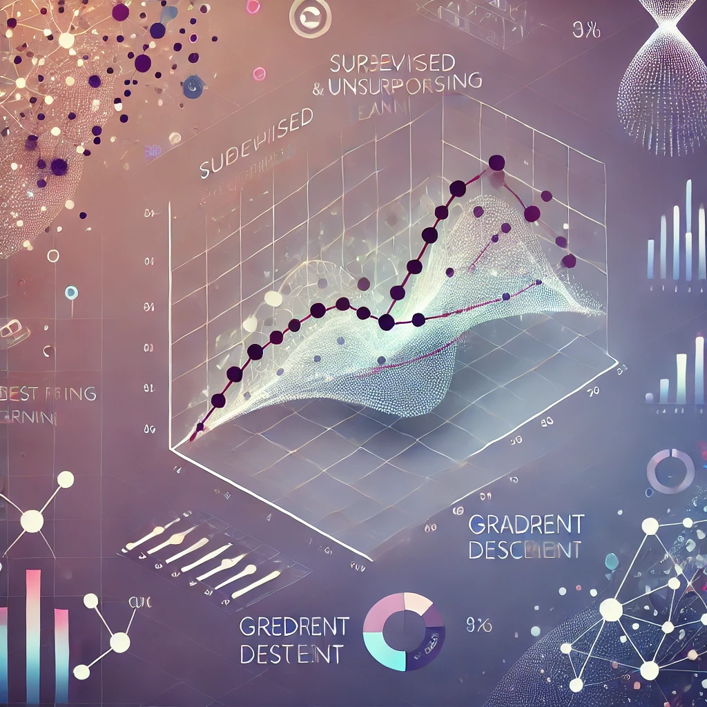
In the realm of machine learning, there are two main types of learning algorithms, supervised and unsupervised. These two approaches provide different ways to solve problems using data, each with its unique applications and methodologies. In this post, we focus on an introduction to both of these concepts as well as a brief dive into the supervised techniques of linear regression and gradient descent.

Supervised Learning

Supervised learning is like teaching a child with flashcards. You show the child a card with a picture of an apple and tell them it's an apple. Over time, the child learns to identify apples on their own, even when you aren't there to guide them. Similarly, in supervised learning, we provide an algorithm with labeled data inputs paired with the correct outputs. The algorithm then learns to make predictions or classifications based on this data.

Applications of Supervised Learning

Here are some common applications of supervised learning:

Input	Output	Application
Email	Spam or Not Spam	Spam Filtering
Audio	Transcripts	Speech Recognition
English Text	Spanish Text	Machine Translation
User Profile	Ad Click Prediction	Online Advertising
Image/Radar Data	Position of Other Cars	Self-Driving Cars
Product Image	Defect Detection (Yes/No)	Visual Inspection

A Concrete Example: Predicting House Prices

Imagine you're trying to predict the price of a house based on its square footage. You could start by plotting the data and fitting a straight line to it, but perhaps a more complex curve might provide a better fit. The goal of a supervised learning algorithm is to determine the best model—whether a simple line (linear regression) or a more complex curve (polynomial regression) —that can accurately predict the house price based on the square footage.

Classification vs. Regression

Supervised learning can be broadly categorized into two types: classification and regression.

• Classification deals with predicting discrete categories, such as whether an email is spam or not. Although many classification tasks involve binary outcomes (e.g., yes or no), they can also involve multiple classes, such as classifying a tumor as benign, malignant type 1, or malignant type 2.

• Regression, on the other hand, deals with predicting continuous values, such as predicting the price of a house. Unlike classification, which has a limited number of outputs, regression models predict a wide range of possible values.

Training a Supervised Model: Spam Filtering

In training a spam filter, for example, we provide the algorithm with a dataset of emails that are already labeled as spam or not spam. The algorithm learns to identify patterns—such as certain words or the length of the email—that help it classify new, unseen emails as spam or not spam.

Unsupervised Learning

Unsupervised learning is a bit like exploring a new city without a map. You don't have specific labels to guide you; instead, you rely on discovering patterns on your own. In unsupervised learning, the algorithm is not provided with labeled data. Instead, it tries to find patterns and relationships in the data on its own.

Another example might be that you're given a task to organize several books in a library. Understandably, you would start to sort the books by things like author and genre. No one told you to organize by these features, you just figured that it was a good idea.

Clustering: Finding Groups in Data

One common application of unsupervised learning is clustering. Here, the algorithm groups data points together based on similarities it finds in the data.

For example, Google News uses clustering algorithms to group stories with similar features together, like stories about pandas that share keywords like "panda," "twin," and "zoo."

Other Applications of Unsupervised Learning

• Anomaly Detection: Identifying unusual data points that do not fit with the rest of the data. This is widely used in fraud detection.
• Dimensionality Reduction: Reducing the number of features in a dataset to make analysis more computationally efficient. This is especially useful in fields like image recognition, where the data might have thousands of features (e.g., pixels).

Visualizing DNA Arrays

A more complex example of unsupervised learning is analyzing DNA arrays. In this case, the algorithm is tasked with identifying genetic patterns without any prior knowledge. The goal is to find similarities and groupings within the genetic data.

Linear Regression in Supervised Learning

Linear regression is one of the foundational techniques in supervised learning, particularly useful for predicting continuous outcomes. The basic idea behind linear regression is to find the best-fitting straight line through a set of data points on a graph. This line represents the relationship between the input features (independent variables) and the output (dependent variable).

The Linear Regression Model

The linear regression model assumes a linear relationship between the input variables and the output. For a simple linear regression with one feature (sometimes referred to as univariate linear regression), the model can be represented as:

$\hat{y} = wx + b$

Here,

• $\hat{y}$ is the predicted output,
• $w$ is the weight (slope) of the line,
• $x$ is the input feature, and
• $b$ is the bias (y-intercept) of the line.

The goal of linear regression is to find the values of $w$ and $b$ that minimize the difference between the predicted outputs $\hat{y}$ and the actual outputs $y$.

Mathletes like myself might also recognize that this resembles the slope intercept form we all learned in middle school

Implement linear regression with Numpy

import numpy as np

# Input data (square footage) and output data (house prices)
x = np.array([1500, 1600, 1700, 1800, 1900, 2000])
y = np.array([300000, 320000, 340000, 360000, 380000, 400000])

# Number of examples
m = len(y)

# Adding a column of ones to X to account for the bias term (intercept)
X = np.c_[np.ones(m), x]

# Initialize the weights (w and b)
theta = np.zeros(2)

# Learning rate and number of iterations
alpha = 0.01
iterations = 1000

# Gradient Descent
for i in range(iterations):
    predictions = X.dot(theta)
    errors = predictions - y
    theta = theta - (alpha / m) * X.T.dot(errors)

# Final parameters
print(f"Final parameters: w = {theta[1]:.2f}, b = {theta[0]:.2f}")

Final parameters: w = 34.16, b = 349984.89

The Cost Function

To measure how well a particular line fits the data, we use a cost function. The cost function quantifies the difference between the predicted values $\hat{y}$ and the actual values $y$ across all the training examples. For linear regression, the most commonly used cost function is the Mean Squared Error (MSE), also known as the Squared Error Cost Function. It is defined as:

$J(w, b) = \frac{1}{2m} \sum_{i=1}^{m} \left( \hat{y}^{(i)} - y^{(i)} \right)^2 = \frac{1}{2m} \sum_{i=1}^{m} \left( f_{w,b}(x^{(i)}) - y^{(i)} \right)^2$

Where:

• $m$ is the number of training examples,
• $\hat{y}^{(i)} = f_{w,b}(x^{(i)})$ is the predicted value for the $i$th example,
• $y^{(i)}$ is the actual value for the ith example.

The factor $\frac{1}{2}$ is included for mathematical convenience, as it simplifies the derivative calculations during gradient descent.

In the following image, $\hat{y}$ is where the predicted value is while $y$ is where the actual value is

Gradient Descent: Finding the Best Fit

Gradient descent is an optimization algorithm used to minimize the cost function. Imagine standing on a hilly golf course, and you want to find the quickest path to the lowest point. Gradient descent helps you find the best direction to move in at each step to reach that lowest point.

The Gradient Descent Algorithm

Gradient descent updates the parameters $w$ and $b$ using the following update rules:

$w := w - \alpha \frac{\partial}{\partial w} J(w, b)$

$b := b - \alpha \frac{\partial}{\partial b} J(w, b)$

Where:

• $\alpha$ is the learning rate, which controls the step size of the update,
• $\frac{\partial}{\partial w} J(w, b)$ and $\frac{\partial}{\partial b} J(w, b)$ are the partial derivatives of the cost function with respect to $w$ and $b$, respectively.

These partial derivatives are calculated as follows:

$\frac{\partial}{\partial w} J(w, b) = \frac{1}{m} \sum_{i=1}^{m} \left( \hat{y}^{(i)} - y^{(i)} \right) x^{(i)}$

$\frac{\partial}{\partial b} J(w, b) = \frac{1}{m} \sum_{i=1}^{m} \left( \hat{y}^{(i)} - y^{(i)} \right)$

Intuition Behind Gradient Descent

The intuition behind gradient descent is analogous to descending a hill. Imagine you're at the top of a hill and want to reach the lowest point (the minimum cost). At each step, you look around and choose the direction that leads downhill (negative gradient) and take a step proportional to the slope of the hill. This process is repeated until you reach the bottom, where the slope (gradient) is zero.

In the context of linear regression, the "hill" represents the cost function $J(w, b)$, and the gradient tells us how to adjust $w$ and $b$ to reduce the cost.

Choosing the Learning Rate

The learning rate $\alpha$ is crucial in gradient descent. If $\alpha$ is too small, the algorithm will take tiny steps and converge slowly. If $\alpha$ is too large, the algorithm might overshoot the minimum and fail to converge. It's essential to choose an appropriate learning rate to ensure efficient and effective optimization.

Convergence of Gradient Descent

Gradient descent is considered to have converged when the change in the cost function between iterations becomes negligibly small. This indicates that the parameters $w$ and $b$ have reached values that minimize the cost function.

In practice, we often monitor the cost function $J(w, b)$ over iterations and stop the algorithm when the cost stops decreasing significantly or when a predefined number of iterations is reached.

Visualizing Gradient Descent

To visualize the process of gradient descent, consider a contour plot of the cost function. The contour lines represent points with equal cost. Gradient descent moves the parameters $w$ and $b$ in the direction of the steepest decrease in cost, eventually converging to the point where the cost is minimized.

For example, in a contour plot of $J(w, b)$, the minimum point (global minimum) would be at the center of the innermost contour line, where the cost is the lowest.

The Importance of Feature Scaling

In some cases, the features in your dataset might have different scales. For example, the square footage of a house might be in the thousands, while the number of bedrooms is in single digits. This can make it difficult for the algorithm to learn effectively. Feature scaling is a technique used to normalize the range of independent variables or features of data.

Techniques for Feature Scaling

• Basic Scaling: Dividing by the maximum value.
• Mean Normalization: Adjusting the values based on the mean and range.
• Z-Score Normalization: Adjusting based on the mean and standard deviation.

Feature Engineering

Feature engineering involves creating new features from existing ones to improve the performance of your model. For example, if you’re predicting house prices, you might create a new feature by multiplying the width and depth of a house to get its area.

Polynomial Regression

Sometimes, the relationship between the input and output isn’t linear. Polynomial regression is used in such cases, fitting a curve instead of a straight line. This allows the model to capture more complex patterns in the data.

Conclusion

Understanding the difference between supervised and unsupervised learning is crucial in choosing the right approach for your problem. Whether you're classifying emails or grouping news stories, the choice of algorithm and techniques like feature scaling and engineering can make a significant impact on the success of your machine learning model.